Time Between The Lines: how memory access affects performance

As programmers, one of our main jobs is to reason about algorithms and put them to use. And one of the tools we use for this task is complexity analysis. Measured in “Big O” notation, an algorithm’s complexity gives us a rough idea of how quickly it performs in the face of different input sizes. For example, we learn that inserting an item into the middle of a linked list is a constant time (O(1)) operation, while inserting into the middle of an array is done in linear time (O(n)), since we must move all subsequent items over to make room. Analysis like this allows us to make informed decisions about how to design our programs. But classical complexity analysis usually comes with an assumption — that all memory access is created equal. On modern hardware, this just isn’t true. In fact, it is extremely false.

Memory hierarchies and you

In the beginning, all hardware was slow. But that was okay — really smart people were able to do some great stuff with it, like land people on the moon with a 2 MHz CPU and 4 kilobytes of RAM.

Apollo 11 moon walk — One small step for man, one giant leap for integrated circuits

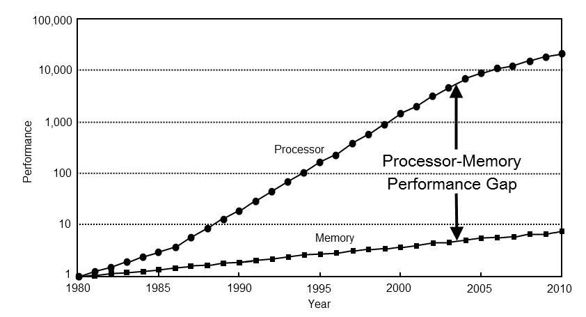
Meanwhile, this guy named Moore predicted that computer designs would speed up at an exponential rate, and as luck would have it, he was right. New processors went faster and faster, and so did memory. But CPU advancements outpaced memory ones, and this started to become problematic. Even though both were quicker than ever before, the processor had to wait more and more cycles to to get data from memory. And having the processor sit around doing nothing is not good for performance.

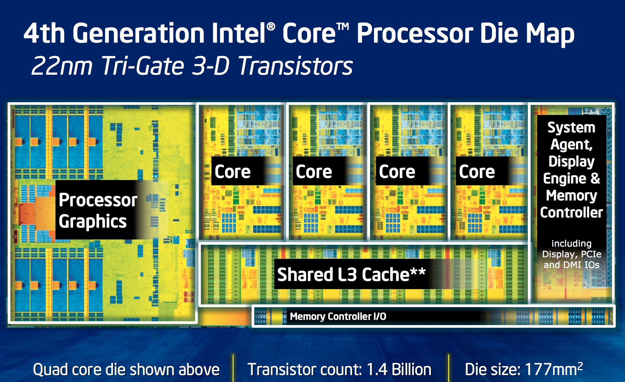
Processor vs. memory speeds — Computer Architecture: A Quantitative Approach by John L. Hennessy, David A. Patterson, Andrea C. Arpaci-Dusseau

So hardware engineers took some RAM and put it directly onto the CPU die so it could be accessed faster. Now we had a two-layered system. When the processor needed something from memory, it would first check this on-die cache. There is a good chance a program will use the same memory repeatedly, so over the entire run we save a lot of time. This works so well that hardware designers started adding a cache for the cache, and then a cache for the cache’s cache. These days it isn’t uncommon for desktop CPUs to have level 1, 2, and 3 caches that take up a good portion of a CPU die.

Haswell die map — A die map of an Intel Haswell processor. Note that a good part of each core is also L1 and L2 cache.

Prefetching

Hardware designers had one more trick up their sleeves. (Well, they actually have a lot of tricks, but those are for another day.) They noticed that a program accessing some part of memory is likely to access nearby memory next. This concept is often called spatial locality. So, if we have to go out to main memory due to a cache miss, we can save time down the road by fetching some adjacent data to put in the cache along with what we need right now. This is known as prefetching.

Why do we care?

This knowledge carries a massive consequence: the order in which a program accesses memory has an impact on how fast our program runs. Accessing memory sequentially will be faster than any other kind of memory access. Just how much faster? Let’s run some experiments.

Assumptions and disclaimers

You may (correctly) get the idea that modern processors are extremely complicated and play all sorts of trickery to squeeze more performance out of your code. This makes timing and benchmarking them tricky to do accurately. For the following experiments, I try to minimize the number of undesired variables with the following steps. Let me know if you think I missed something big.

To start each run with an “empty” CPU cache that contains no data related to the experiment, we “clear” it by copying an unrelated buffer as large as the cache before a trial run. This should fill the cache with the dummy buffer’s data, forcing the CPU to to initially fetch all our experiment data from main memory.
To minimize the impact of other processes and the operating system on our metrics, we
- Avoid running other processes during the experiment as much as possible.
- Perform no I/O (which could cause stalls while waiting for the related device to become ready).
- Perform a large number of trials (generally a good idea in any experiment).
- Have each experiment take a substantial amount of time (at least to a computer), hopefully averaging out irregularities caused by being interrupted.
- Use a system-provided, high resolution clock for our measurements.

The base case

Note: Code snippets here are edited for brevity. You can find the complete source for the experiments on Github.

For each of the experiments, let’s create a list of integers much larger than the cache so we can see how cache misses affect performance. My processor is an Intel Core i7 4790k with 8MB of cache, so I’ll use 80 MB of integers. Let’s initialize these integers with some random values (here in the range 1–10), clear the cache, start the clock, then do some arbitrary work on the data. Here we average the squares of all the values in the list.

int doWork(const vector<int>& data)
{
	unsigned long sum = 0;

	for (int d : data)
		sum += d * d;

	return (int)(sum / data.size());
}

We will record how long that run took, and once we have finished all our runs, average these trial times.

for (unsigned int i = 0; i < iterations; ++i) {
	populateDataSet(data, rng);
	clearCache();

	const auto runStart = clk::now();
	const int result = doWork(data);
	const auto runTime = clk::now() - runStart;
	runSum += runTime;
	// We write out the result to make sure the compiler doesn't
	// eliminate the work as a dead store,
	// and to give us something to look at.
	cout << "Run " << i + 1 << ": " << result << "\r";
	cout.flush();
}

The only thing we will change for each experiment is the way the data is accessed. For our first experiment, let’s access the data directly, in sequential order. Our knowledge of prefetching tells us that this should be our fastest case. I get:

$ g++ -Wall -Wextra -std=c++14 -O2 -o base base.cpp
$ ./base
Run 1000: 38
Ran for a total of 300.632 seconds (including bookkeeping and cache clearing)
1000 runs took 10.444 seconds total,
Averaging 10.444 milliseconds per run

So, that’s a base case of about 10.4 milliseconds to average 80 MB of integers.

Case 2: Now with indirection

Unfortunately, some languages do not allow you to store values directly in a contiguous array (at least not for user-defined types). Instead, they use references, so our array becomes an array of pointers. In the best case, the actual data they point to is allocated in sequential order, so our only performance hit is the indirection. To simulate this, let’s operate on an array of pointers to the data instead of operating on the data directly.

int doWork(const vector<int*>& data)
{
	unsigned long sum = 0;

	for (int* d : data)
		sum += *d * *d;

	return (int)(sum / data.size());
}

// Before the trials,
auto pointers = vector<int*>(data.size());
for (size_t i = 0; i < data.size(); ++i)
    pointers[i] = &data[i];
}

Let’s try that:

$ g++ -Wall -Wextra -std=c++14 -O2 -o indirection indirection.cpp
$ ./indirection
Run 1000: 38
Ran for a total of 304.947 seconds (including bookkeeping and cache clearing)
1000 runs took 12.860 seconds total,
Averaging 12.860 milliseconds per run

We notice that performance is just a bit slower because some of our cache space is taken up by the pointers.

Case 3: Non-contiguous allocations

Our assumption from case 2 that separate allocations will be placed in contiguous memory locations is a poor one. Maybe adjacent memory is taken up by some other allocations from our program. Also, some allocators will intentionally allocate memory in pseudo-random locations for security reasons and so out of bounds access generates a page fault instead of silently breaking things. To simulate this, we will repeat our processes from case 2, but will shuffle the pointers between each run.

// Before each run,
shuffle(begin(pointers), end(pointers), rng);

This will be the worst of our cases, since all the non-contiguous access means prefetching is almost completely ineffective.

$ g++ -Wall -Wextra -std=c++14 -O2 -o random random.cpp
$ ./random
Run 1000: 38
Ran for a total of 1194.71 seconds (including bookkeeping and cache clearing)
1000 runs took 164.585 seconds total,
Averaging 164.585 milliseconds per run

Oof. Just by doing the same work in a different order, we are an order of magnitude slower.

It’s (probably) actually worse

These experiments are pretty simplistic approximations of memory access in “real” programs, which might be even worse. When working on data larger or of a more complex type than a meager integer, each element will be farther apart, so the memory architecture can’t prefetch as many elements at once. And data structures besides arrays tend to use more indirection, being less cache-friendly out of the gate.

Big lessons

Our biggest takeaway is that how you arrange and access your memory has huge performance ramifications. In more practical terms,

You get massive, “free” performance boosts by placing data that is used together close together in memory. Consider entities in some hypothetical game engine:

class GameEntity {
    AIComponent ai;
    PhysicsComponent physics;
    RenderComponent render;
};

// Elsewhere...
vector<GameEntity> entities;

// Elsewhere...
// (Hilairously oversimplified) main game loop
for (auto& ge : entities) {
    ge.ai.update();
    ge.physics.update();
    ge.render.draw();
}

If the calculations for AI components access other AI components, the physics components access other physics components, and so on, we can speed things up by getting these respective components closer to each other in memory:

class GameEntity {
    AIComponent* ai;
    PhysicsComponent* physics;
    RenderComponent* render;
};

// Elsewhere...
vector<GameEntity> entities;
vector<AIComponent> aiComponents;
vector<PhysicsComponent> physicsComponents;
vector<RenderComponent> renderComponents;

// Elsewhere...
// (Hilairously oversimplified) main game loops
for (auto& a : aiComponents) { a.update(); }
for (auto& p : physicsComponents) { p.update(); }
for (auto& r : renderComponents) { r.draw(); }

Such a small change can reap huge performance benefits. This is not to say that you should try to shoehorn everything into an array when the situation calls for another data structure, but look out for opportunities like the one shown here.

When choosing an algorithm or data structure, take its memory access patterns into account. Doing more work that causes fewer cache misses can be faster. Complexity analysis is only a rough guide to performance. Let’s revisit our original discussion comparing linked lists to arrays. On paper, removing from the middle of an array should take take much longer than removing from the middle of a linked list. But if you must first traverse the list to find the item, a traversal and removal from an array actually scales much better than a traversal and removal from a linked list due the cache-friendliness of an array.

Memory matters. Any serious optimization efforts must take it into account, lest your processor sit around waiting on cache misses.