Simulating Airband AM Radios

In a slight departure from what I usually talk about here, let’s chat about airplane radios.

For the last several years, I’ve spent most Saturdays playing (and occasionally working on) BMS, a modern¹ combat flight sim where you fly virtual F-16s around with friends and blow stuff up. Any co-op game with over 30 people is a blast, but air combat is especially fun because it’s such a team sport. Flights swirl in vicious dogfights and play deadly games of whack-a-mole with enemy air defenses, all just to give a few jets a couple of seconds over the target to drop their bombs. None of it is scripted, and everyone has to do their job to come back alive.

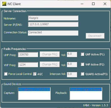
You might imagine this involves a lot of talking, and so BMS ships with a voice chat app called IVC. To add to the immersion, it simulates the radios in your virtual cockpit. You don’t join a chat room, you tune to a radio frequency. Your signal fades as your jet gets further from whoever you’re talking to, or if you’re both flying low, you can be blocked by terrain entirely.

Surprisingly, airplane radios—even many military ones—are still simple AM sets which transmit in the VHF and UHF bands. One of the reasons that’s persisted through decades of technological advances is that AM radio doesn’t have a “capture effect”. When two people talk over each other on the same frequency, you can still hear both parties, unlike FM where the louder signal mutes or “captures” the quieter one. Here’s what it sounds like when some fighter pilots talk over each other, captured during a Red Flag training exercise in Nevada:

So imagine my… curiosity when IVC sounds like this whenever players talk on the same frequency:

That bugs me more than it should. So when a buddy set out to build an IVC replacement with better UX and modern audio codecs, I wanted to contribute some realistic AM radio dynamics. Let’s dive in.

Radio 101: path loss, decibels, SNR

So you want to talk to someone over the radio. Let’s set aside the black magic of antenna design—take it as a given that if you cut the right length of wire and wiggle the electrons in it, some of them will magically shear off into space as electromagnetic waves. Even if those waves don’t run into anything,² they get weaker as a square of radius $r$ from the transmitting antenna, simply because they spread out as they travel.

This is true of all waves—sound, radio, light.³ And because different distances from the source produce such wildly different power levels, our senses need to work on logarithmic scales. They’re actually pretty astonishing—the roar of a jet engine is a million times louder than the quietest whisper, and you can hear both. A room can be a million times darker than a sunny day, yet you can see in both.

The radio frequency (RF) world is no different. Because it would be annoying to work with such a wide range of numbers, we often describe signal strength in a logarithmic scale called decibels, abbreviated as dB. One of the first things we’d like to describe in decibels is the signal-to-noise ratio, or SNR.

Some noise is man-made, some comes from atmospheric events like thunderstorms, and some comes from outer space. More noise comes from the imperfections in your radio’s electrical components. And even if you could somehow remove all of those noises, you’d still hear thermal energy vibrating the electrons in your receiver. (We call this phenomenon thermal noise and it’s our theoretical minimum.)

But no matter where it comes from, noise is always there! We can never get rid of it; we only hope the received signal is louder than the noise by the time it reaches us.

Amplitude modulation

So what waves should you broadcast? The frequencies that make up your voice (and everything else you hear) are between 20 and 20,000 cycles per second, or Hertz. But the lower the frequency, the longer the wavelength, and good antennas are at least a quarter of the wavelength they receive. To pick up a 10 kHz signal, we’d need over 7 kilometers of wire.⁴

Instead, let’s shift our voice onto some higher carrier frequency that we can actually transmit. A simple approach is to modulate the carrier wave’s amplitude by that of our voice. We might call this amplitude modulation, or AM for short.

Notice how the outlined shape of the resulting AM signal—its envelope—is a mirrored copy of our voice. Hmm…

What’s in a radio?

Glossing over how you tune your radio to different frequencies (the answer might shock you!), we have a few other problems to solve if we want to hear an AM signal:

1. We need to filter out all the frequencies we don’t care about, passing only the band of frequencies we actually want. (Let’s call that the passband.)

2. The signal is probably very weak by the time we get it (see above), so we need to amplify it.

3. Lastly, we use an envelope detector to extract, or demodulate, our voice back out of the AM signal.

Filtering

How do we let some frequencies through and block others out? Let’s talk circuits 101.

In the analog world, we deal in:

• Current (I), which represents electrons flowing through our circuit
• Voltage (V), which represents the electric potential energy between two parts of a circuit, and
• Resistance (R), which represents the reluctance of some part of a circuit to let current flow through it.

They can behave in unintuitive ways, but they are always proportional to each other according to Ohm’s law:

With this knowledge, we can make one of the simplest useful analog circuits: a voltage divider.

The squiggly bits represent resistors, and the inverted dashed triangle at the bottom represents ground, or 0 volts, to which we compare all our other voltages. Because resistors oppose the flow of current, our output voltage will be some fraction of the input voltage, based on the ratio of the two resistors. Drag the slider to change that ratio, and observe how:

What if we swap out one of the resistors for something more interesting?

This symbol represents a capacitor, a part that stores electric charge between two plates, and can discharge it later. If we swap $R_2$ out for one, we get the behavior:

As time $t$ goes by, $V_{out}$ asymptotically approaches $V_{in}$ at a rate determined by the resistance $R$ multiplied by the capacitance $C$. Because of this, we call $RC$ the time constant, or $\tau$. A little more math shows us that every $3 \tau$, the voltage advances 95% of the way from $V_0$ to $V_{in}$, where $V_0$ is just whatever our starting voltage was.

This makes capacitors useful for all sorts of applications, but the thing we care about today is how one behaves when given an alternating input (like a wave from an antenna!) instead of a constant one. Because the capacitor is constantly charging and discharging, its resistance⁵ decreases as frequency increases. This makes our RC circuit a low-pass filter that lets low frequencies through and shrinks—or attenuates—high frequencies.

And if we just swap the resistor and capacitor, we have a high-pass filter. Instead of the capacitor shunting high frequencies to ground, it’s letting high frequencies through from $V_{in}$, and so low frequencies are attenuated.

Filter design can get amazingly complex—there are whole textbooks on this stuff—but the basics don’t have to be. We’ll find that it’s surprisingly easy to do this in the digital world as well.

Automatic gain control

We also need to amplify our signal. But how much? Even though we’ll receive signals with wildly different strengths, it would be great if our radio had a consistent volume level when someone is talking. We want to control the amplification, or gain, automatically.

How do we do that? More filters! If we take the magnitude of our signal, then low-pass it, we end up with a curve that gives a rough measure of its volume.

We have a slight conundrum, though—we want the filter to respond quickly when someone starts talking, but to taper off slowly, so that the measured volume doesn’t drop whenever they pause to take a breath. To do this we build a filter that responds differently when the signal rises (call this attack) and when the signal falls (call this decay).

I also added a period of silence to our AM transmission—after all, pilots aren’t talking on the radio 100% of the time. Try moving the sliders around until the filtered magnitude:

• Rises to the peak volume quickly when a transmission starts
• Stays flat-ish for the entire transmission, but
• Decays back to 0 quickly-ish when the transmission stops

And lo, you’ve measured the volume of our signal! If we divide whatever comes in by this value, the user should always hear a similar volume.

AM demodulation

Notice how if you drag the sliders around some more, we get something that looks suspiciously like the envelope. In fact, this sort of filter is sometimes called an “envelope detector”. To demodulate our AM signal back into the transmitted voice, we just need to low-pass the signal with one of them.

Squelch

Scroll back up to our SNR demo, and drag the slider all the way to the left until you hear only static. Isn’t that unpleasant? Nobody likes hearing static for extended periods of time, so radios quickly grew a feature called squelch, which mutes your speakers whenever the signal falls below a certain volume. Good thing we just came up with a way to measure it!

Drag the sliders around and consider some of the interesting effects going on:

1. When you turn the SNR down to about 0 dB, our transmission is no louder than the noise, and the squelch gate mutes us. But turn down the squelch threshold and you can still make things out! For this reason, some radios provide a way to disable squelch so you can listen to weak signals.

2. If you’ve listened to airband radios before, you’re probably familiar with a “click” when someone starts talking and a “kssh” when they stop. This isn’t some artificial sound effect—it’s a natural product of the interplay between AGC and squelch. As a transmission starts and the measured volume shoots above the noise floor, the squelch gate flies open as AGC quickly moves to attenuate the signal. The resulting pop, constrained by our bandwidth, softens to a clicking noise. (Try it with and without the bandpass.) Then, when the transmission stops, AGC rapidly turns the volume back up, so we hear the static rush in before the squelch gate clicks back off.

Whenever you’re done with the demo, just drag squelch back up above the noise floor. Remember, noise is always there!

Interference

With those basics out of the way, let’s get back to that interference we hear when several folks talk at once. Where do all those funny noises come from?

We don’t live in an ideal world, and our electronics are no exception. If I tune my radio to 121.5 MHz, its carrier frequency is oscillating back and forth 121.5 million times a second. That’s pretty impressive! But I shouldn’t be surprised if it’s not exactly that many Hertz. Without very expensive machinery, electronic oscillators drift a little bit, especially as they heat and cool (which airplanes tend to do when they fly around).

Additionally, whenever someone is moving, the Doppler Effect shifts the frequency of anything they transmit. If they’re going several hundred knots in a fighter jet, this shift can be substantial. (In fact, one of the revolutions in airborne radars was to measure this frequency shift, and use it to separate a plane on the radar screen from all the background clutter behind it. A fun story for another day!)

What’s really neat is that an AM receiver usually doesn’t care. If you think you’re tuned to 121.5 MHz, but you’re actually on 121.4999 MHz, or receiving a signal at 121.5001 MHz, the envelope detector still demodulates the exact same envelope, and we’re good to go. That is until several people start talking.

Whenever frequency $A$ is played at the same time as frequency $B$, they create a beat frequency at $|B - A|$.

You’ve heard this yourself if you’ve ever tuned a musical instrument.

This same effect occurs with our imperfectly-tuned radios—while the carrier frequencies themselves are hundreds of times higher than the bandwidths of both the radio and your ears, the beats are not! One transmitter at 121.499 MHz and another at 121.501 MHz gives us a very audible, and very annoying, 2 kHz whine. You can listen to it and other example tones at https://www.szynalski.com/tone-generator/.

These beats also cause strange things to happen to the envelope:

• Voices are ring-modulated by the beat frequencies. (Think Daleks.)

• Louder voices amplitude modulate weaker ones.

• In severe cases, the envelope rises and falls rapidly, causing the AGC to rapidly “pump” the volume.

We’ll see why soon.

Again! But with computer!

Next we need to make a computer do all of that.

For starters, computers (except the quantum ones) don’t deal in continuous analog values. Instead, when we want to record some audio, an analog-to-digital converter samples the voltage of a microphone over and over, thousands of times a second, into numbers that form a connect-the-dots representation of the sound waves. Your computer can also do the opposite—a digital-to-analog converter can turn a big list of numbers back into voltages that shake the diaphragm of your speakers. If we want to do any digital signal processing in between, we’re just transforming long lists of numbers into slightly different lists of numbers.

About 100 years ago, some very smart people figured out you need double the sample rate of the frequencies you care to represent.

And since human hearing tops out around 20 kHz, sample rates of 44.1 kHz⁶ and 48 kHz are common for digital audio. This is fortunate for us because “48 thousand times a second” is pretty trivial on a modern CPU.

Filtering

Recall the voltage equation for our RC filter:

It doesn’t look too different in the digital world, where given some list of samples $x[n]$, each output $y[n]$ is calculated from the current sample and the previous output:

where for a sample period $T$, or sample rate $F_s$

If you want an envelope filter with separate attack and decay coefficients, pick a different $\tau$ depending on whether $x[n] \geq y[n-1]$. We’ll use this for our AGC.

Just like in the analog world, digital filter design can get much more complicated, but we can start here.

IQ sampling

In a similar way, we can directly calculate the sound of multiple transmitters interfering with each other. But to do that, we need to chat some more about how we represent frequencies in the first place. All the waves we’ve looked at so far have been a single sinusoid wiggling up and down. That’s a simple representation, but it’s a bit lacking. For starters, it’s ambiguous—at most points in time, you can’t determine the phase of the signal.

What if instead we represented a frequency with two sinusoids—both a cosine and a sine?

Because the sine wave is a quarter cycle behind the cosine, we often call this representation “in-phase and quadrature encoding”, or IQ for short.

So instead of thinking about a frequency as a single wave moving up and down at a given rate, imagine it as a phasor spinning around at that rate:

Phasors can also spin the opposite way, giving us a negative frequency. If this notion seems weird and scary to you, you’re not alone! It was a long time before any negative numbers stopped seeming weird to mathematicians.

Since RF engineers work with IQ a lot, they want a more concise way to express phasors. If we turn a phasor into a complex number, then we can use Euler’s formula to represent it as a single term, $e$ raised to an imaginary⁷ exponent:

(In the electrical engineering world, we use $j = \sqrt{-1}$ instead of $i$ because $i$ represents current.)

We won’t use that formulation much today, but it’s everywhere in the signal processing world. If you want to learn more, check out the DSP GOAT Richard Lyons’s explanation, Quadrature Signals: Complex, But Not Complicated.

A baseband AM simulation

Now we’re ready to put it all together. We’re going to simulate our AM radios in baseband—i.e., only the audio frequencies that would be demodulated by the envelope detector. The main reason for this is that a full band simulation of the carrier frequencies at over 100 MHz would be difficult to do in real time, since we’d have to process hundreds of millions of samples each second.

For $m$ radios transmitting at once on carrier frequencies $C_1, C_2, \cdots, C_m$, we’ll make a list of relative frequencies $F_m = C_m - C_1$. Note how an arbitrary frequency—the first in our list, $C_1$—becomes our “zero” frequency. In the digital world with a sample rate $F_s$, this means our phase angle for each is:

We can then represent each of our signals as a product of that phasor, its $\text{SNR}_m$, and its samples $x_m[n]$ multiplied by our modulation index $k$.

The single signal case is pretty boring: $F_1 = 0$, and since $\cos(0) = 1$ and $\sin(0) = 0$, this simplifies to:

Subsequent transmitters get a bit more interesting. Their phase $\theta$ isn’t 0—instead it’s rotating at $F_m$. For example, if our first signal had a 100 MHz carrier and our second had a 100.002 MHz carrier, we’d get a $\theta$ rotating at 2 kHz. Repeat this for each transmitter, throw in some random noise $(R_I[n], R_Q[n])$ for good measure, and all of these IQ vectors sum to

Our audible envelope is just the length of that IQ vector:

$E[n] = \sqrt{I[n]^2 + Q[n]^2}$.

If you plot this out, you start to see the wackiness. While the first signal—which we’re calculating everything relative to—is always in-phase with itself, the other signals constantly shift in phase, producing the effects we discussed earlier.

Feed that into our AGC filter, squelch the output when $\text{AGC}[n]$ is less than our threshold, apply a bandpass filter to limit it to AM bandwidths (about 300 Hz to 3–5 kHz), and we’re done! The results sound pretty cool. Here’s a snippet from an old demo:

What’s even cooler is that there’s not a lot to tweak. Our only real inputs are:

• Our signals and their relative strengths
• Some randomly-generated noise
• Attack and decay constants for our AGC
• Upper and lower band limits for our bandpass filter

And from that we get a simulation that 4 out of 4 dentists pilots say sounds just like the real deal. I think there’s a valuable lesson there—while your sim will never be exactly like real life, you can get surprisingly close with surprisingly little code if you sit and think about the problem from first principles.

You can grab a copy of that demo app to mess around here, or check out the actual code here. Cheers!